Strange Attractors | Shashank Tomar

A few months back, while playing around with , I came across something that completely derailed my plans. Strange attractors – fancy math that creates beautiful patterns. At first I thought I’d just render one and move on, but then soon I realized that this is too much fun. When complexity emerges from three simple equations, when you see something chaotic emerge into beautiful, it’s hard not to waste some time. I’ve spent countless hours, maybe more than I’d care to admit, watching these patterns form. I realized there’s something deeply satisfying about seeing order emerge from randomness. Let me show you what kept me hooked.

The Basics: Dynamical Systems and Chaos Theory

Dynamical Systems are a mathematical way to understand how things change over time. Imagine you have a system, which
could be anything from the movement of planets to the growth of a population. In this system, there are rules that
determine how it evolves from one moment to the next. These rules tell you what will happen next based on what is
happening now. Some examples are, a pendulum, the weather patterns, a flock of birds, the spread of a virus in a
population (we are all too familiar with this one), and stock market.

There are two primary things to understand about this system:

• Phase Space: This is like a big collection of all the possible states the system can be in. Each state is like a
  snapshot of the system at a specific time. This is also called the state space or the world state.
• Dynamics: These are the rules that takes one state of the system and moves it to the next state. It can be
  represented as a function that transforms the system from now to later.

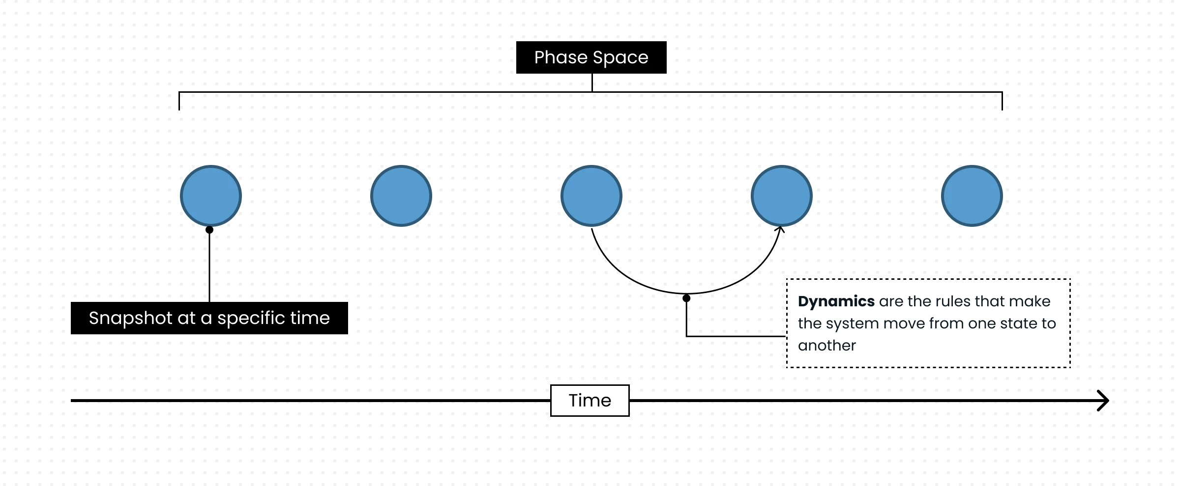
Figure 1 – Phase Space in Dynamical Systems

For instance, when studying population growth, a phase-space (world-state) might consist of the current population size
and the rate of growth or decline at a specific time. The dynamics would then be derived from models of population
dynamics, which, considering factors like birth rates, death rates, and carrying capacity of the environment, dictate
the changes in population size over time.

Another way of saying this is that the dynamical systems describe how things change over time, in a space of
possibilities, governed by a set of rules. Numerous fields such as biology, physics, economics, and applied mathematics,
study systems like these, focusing on the specific rules that dictate their evolution. These rules are grounded in
relevant theories, such as Newtonian mechanics, fluid dynamics, and mathematics of economics, among others.

Chaos Theory

There are different ways of classifying dynamical systems, and one of the most interesting is the classification into
chaotic and non-chaotic systems. The change over time in non-chaotic systems is more deterministic as compared to
chaotic systems which exhibit randomness and unpredictability.

Chaos Theory is the sub branch of dynamical systems that studies chaotic systems and challenges the traditional
deterministic views of causality. Most of the natural systems we observe are chaotic in nature, like the weather, a drop
of ink dissolving in water, social and economic behaviours etc. In contrast, systems like the movement of planets,
pendulums, and simple harmonic oscillators are extremely predictable and non-chaotic.

Chaos Theory deals with systems that exhibit irregular and unpredictable behavior over time, even though they follow
deterministic rules. Having a set of rules that govern the system, and yet exhibit randomness and unpredictability,
might seem a bit contradictory, but it is because the rules do not always represent the whole system. In fact, most of
the time, these rules are an approximation of the system and that is what leads to the unpredictability. In complex
systems, we do not have enough information to come up with a perfect set of rules. And by using incomplete information
to make predictions, we introduce uncertainty, which amplifies over time, leading to the chaotic behaviour.

Figure 2 – Unpredictability in Chaos Theory

Chaotic systems generally have many non-linear interacting components, which we partially understand (or can partially
observe) and which are very sensitive to small changes. A small change in the initial conditions can lead to a
completely different outcome, a phenomenon known as the butterfly effect. In this post, we will try to see the
butterfly effect in action but before that, let’s talk about Strange Attractors.

Strange Attractors

To understand Strange Attractors, let’s first understand what an attractor is. As discussed earlier, dynamical systems
are all about change over time. During this change, the system moves through different possible states (remember the
phase space jargon?). An attractor is a set of states towards which a system tends to settle over time, or you can say,
towards which it is attracted. It’s like a magnet that pulls the system towards it.

For example, think of a pendulum. When you release it, it swings back and forth, but eventually, it comes to rest at the
bottom. The bottom is the attractor in this case. It’s the state towards which the pendulum is attracted.

This happens due to the system’s inherent dynamics, which govern how states in the phase space change. Here are some of
the reasons why different states get attracted towards attractors:

• Stability: Attractors are stable states of the system, meaning that once the system reaches them, it tends to stay
  there. This stability arises from the system’s dynamics, which push it towards the attractor and keep it there.
• Dissipation: Many dynamical systems have dissipative forces, which cause the system to lose energy over time. This
  loss of energy leads the system to settle into a lower-energy state, which often corresponds to an attractor. This is
  what happens in the case of the pendulum.
• Contraction: In some regions of the phase space, the system’s dynamics cause trajectories to converge. This
  contraction effect means that nearby states will tend to come closer together over time, eventually being drawn
  towards the attractor.

Figure 3 – Attractor state in a simple pendulum

Some attractors have complex governing equations that can create unpredictable trajectories or behaviours. These
nonlinear interactions can result in multiple stable states or periodic orbits, towards which the system evolves. These
complex attractors are categorised as strange attractors. They are called “strange” due to their unique
characteristics.

1. Fractal Structure: Strange attractors often have a fractal-like structure, meaning they display intricate
   patterns that repeat at different scales. This complexity sets them apart from simpler, regular attractors.
2. Sensitive Dependence on Initial Conditions: Systems with strange attractors are highly sensitive to their initial
   conditions. Small changes in the starting point can lead to vastly different long-term behaviors, a phenomenon known
   as the “butterfly effect”.
3. Unpredictable Trajectories: The trajectories on a strange attractor never repeat themselves, exhibiting
   non-periodic motion. The system’s behavior appears random and unpredictable, even though it is governed by
   deterministic rules.
4. Emergent Order from Chaos: Despite their chaotic nature, strange attractors exhibit a form of underlying order.
   Patterns and structures emerge from the seemingly random behavior, revealing the complex dynamics at play.

You can observe most of these characteristics in the visualisation. The one which is most fascinating to observe is the
butterfly effect.

The Butterfly Effect

A butterfly can flutter its wings over a flower in China and cause a hurricane in the Caribbean.

One of the defining features of strange attractors is their sensitivity to initial conditions. This means that small
changes in the starting state of the system can lead to vastly different long-term behaviors, a phenomenon known as the
butterfly effect. In chaotic systems, tiny variations in the initial conditions can amplify over time, leading to
drastically different outcomes.

Figure 3 – A Simplification of The Bufferfly Effect

In our visualisation, let’s observe this behavior on Thomas Attractor. It is governed by the following equations:

3
dx = (-a*x + sin(y)) * dt;
4
dy = (-a*y + sin(z)) * dt;
5
dz = (-a*z + sin(x)) * dt;

3
dx = (-a*x + sin(y)) * dt;
4
dy = (-a*y + sin(z)) * dt;
5
dz = (-a*z + sin(x)) * dt;

A small change in the parameter a can lead to vastly different particle trajectories and the overall shape of the
attractor. Change this value in the control panel and observe the butterfly effect in action.

There is another way of observing the butterfly effect in this visualisation. Change the Initial State from cube to
sphere surface in the control panel and observe how the particles move differently in the two cases. The particles
eventually get attracted to the same states but have different trajectories.

Implementation Details

This visualization required rendering a large number of particles using Three.js. To achieve this efficiently, we used a
technique called ping-pong rendering . This method handles iterative updates of particle systems directly on the GPU,
minimizing data transfers between the CPU and GPU. It utilizes two frame buffer objects (FBOs) that alternate roles: One
stores the current state of particles and render them on the screen, while the other calculates the next state.

Implementation Workflow

1. Setting Up Frame Buffer Objects (FBOs): We start by creating two FBOs, ping and pong, to hold the current and
   next state of particles. These buffers store data such as particle positions in RGBA channels, making efficient use
   of GPU resources.

   typescript

   1
   const ping = new THREE.WebGLRenderTarget(size, size, {
   2
     minFilter: THREE.NearestFilter,
   3
     magFilter: THREE.NearestFilter,
   4
     format: THREE.RGBAFormat,
   9
   const pong = new THREE.WebGLRenderTarget(size, size, {
   10
     minFilter: THREE.NearestFilter,
   11
     magFilter: THREE.NearestFilter,
   12
     format: THREE.RGBAFormat,
   14
     type: THREE.FloatType,

   1
   const ping = new THREE.WebGLRenderTarget(size, size, {
   2
     minFilter: THREE.NearestFilter,
   3
     magFilter: THREE.NearestFilter,
   4
     format: THREE.RGBAFormat,
   9
   const pong = new THREE.WebGLRenderTarget(size, size, {
   10
     minFilter: THREE.NearestFilter,
   11
     magFilter: THREE.NearestFilter,
   12
     format: THREE.RGBAFormat,
   14
     type: THREE.FloatType,

2. Shader Programs for Particle Dynamics: The shader programs execute on the GPU and apply attractor dynamics to
   each particle. Following is the attractor function which update the particle positions based on the attractor equation.

   glsl

   1
   vec3 attractor(vec3 pos) {
   3
      float x = pos.x, y = pos.y, z = pos.z;
   7
      dx = (-a*x + sin(y)) * dt;
   8
      dy = (-a*y + sin(z)) * dt;
   9
      dz = (-a*z + sin(x)) * dt;
   10
      return vec3(dx, dy, dz);

   1
   vec3 attractor(vec3 pos) {
   3
      float x = pos.x, y = pos.y, z = pos.z;
   7
      dx = (-a*x + sin(y)) * dt;
   8
      dy = (-a*y + sin(z)) * dt;
   9
      dz = (-a*z + sin(x)) * dt;
   10
      return vec3(dx, dy, dz);

3. Rendering and Buffer Swapping: In each frame, the shader computes the new positions based on the attractor’s
   equations and stores them in the inactive buffer. After updating, the roles of the FBOs are swapped: The previously
   inactive buffer becomes active, and vice versa.

   typescript

   1
   const currentTarget = flip ? ping : pong;
   2
   const nextTarget = flip ? pong : ping;
   5
   uniforms.positions.value = currentTarget.texture;
   8
   gl.setRenderTarget(nextTarget);
   10
   gl.render(scene, camera);
   11
   gl.setRenderTarget(null);

   1
   const currentTarget = flip ? ping : pong;
   2
   const nextTarget = flip ? pong : ping;
   5
   uniforms.positions.value = currentTarget.texture;
   8
   gl.setRenderTarget(nextTarget);
   10
   gl.render(scene, camera);
   11
   gl.setRenderTarget(null);

This combination of efficient shader calculations and the ping-pong technique allows us to render the particle system.

If you have any comments, please leave them on . Sooner or later, I will integrate it with the blog.